M1: From Pixels to Meters

That clip up top: the M0 ball box on the broadcast frame, and its position drawing itself onto a real court diagram in meters — live, frame by frame.
M0 left me with a ball track in pixel coordinates, and pixel coordinates mean nothing. "The ball is at (622, 462)" tells you nothing about whether that's a winner down the line or a ball kid's pocket. M1 is the conversion: find the court in the frame, compute the homography, turn pixels into meters.
I expected geometry homework. Here's the twist: the milestone I was braced for turned out to need zero manual input and zero API calls. Tracking a ball — the "solved" problem — needed a human to click on it. Finding the court needed nothing but numpy.
The median trick
The camera doesn't move during a rally (I checked — more below). So if you
take the per-pixel median over the whole clip, anything that moves gets
voted out of existence. One line of numpy — np.median(frames, axis=0) —
and both players are gone, the ball is gone, and the court lines are razor
sharp.
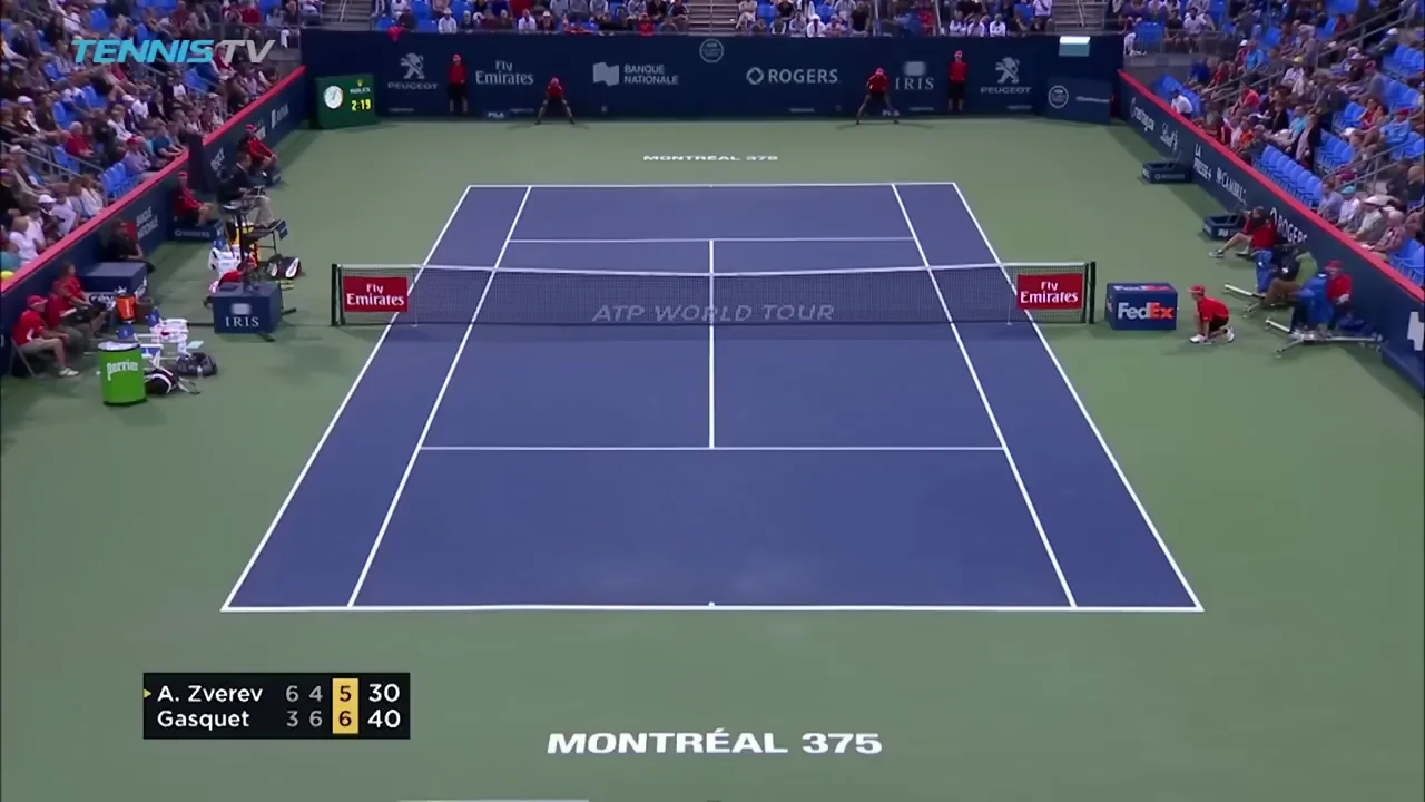
The clean plate — the median over 96 sampled frames. Nobody is playing tennis here, and that's the point.
This also is the static-camera check: if the camera panned even slightly, the median's lines would smear. They don't (edge IoU 0.83 against frame 0, sharpness ratio 0.90), which means one homography serves all 480 frames. The temporal median frame is free player removal. No segmentation model, no inpainting. The line judges leave faint ghosts — they barely move — and the broadcast text overlays survive, but neither matters for what comes next.
Finding the lines
Court lines are white paint on a blue court. So: mask the big blue region (the largest blue contour — 26.5% of the frame), then look for white pixels only inside it. That one restriction keeps the scoreboard, the "MONTRÉAL 375" signage, and the crowd's white shirts out of the line detector entirely.
Run Hough on what's left and you get 48 line segments covering every painted line on the court:
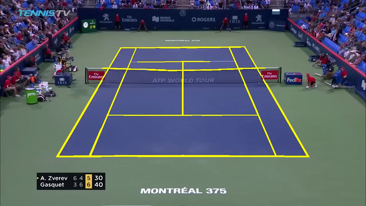
Every court line found — plus one impostor.
The impostor: the net tape reads as a horizontal line too. It's white, it's long, and it's not on the ground. Worse, it sags — it's not even straight. Any naive "match six horizontal lines to the court model" scheme would choke on it.
Four corners are enough
The dodge is embarrassingly simple. Cluster the segments into line families (five horizontal, five vertical) and take only the extremes: topmost and bottommost horizontals are the baselines, leftmost and rightmost verticals are the doubles sidelines. The net sits mid-pack by definition — it can never be an extreme. Intersect those four lines, get four corners, and ask OpenCV for the perspective transform onto a court model that's just the official dimensions: 10.97 by 23.77 meters.
Four corners is the minimum possible input for a homography. Would it be any good? The honest test: the singles sidelines, both service lines, and the center line took no part in the fit. Reproject the full court model through the homography and see where those held-out lines land:
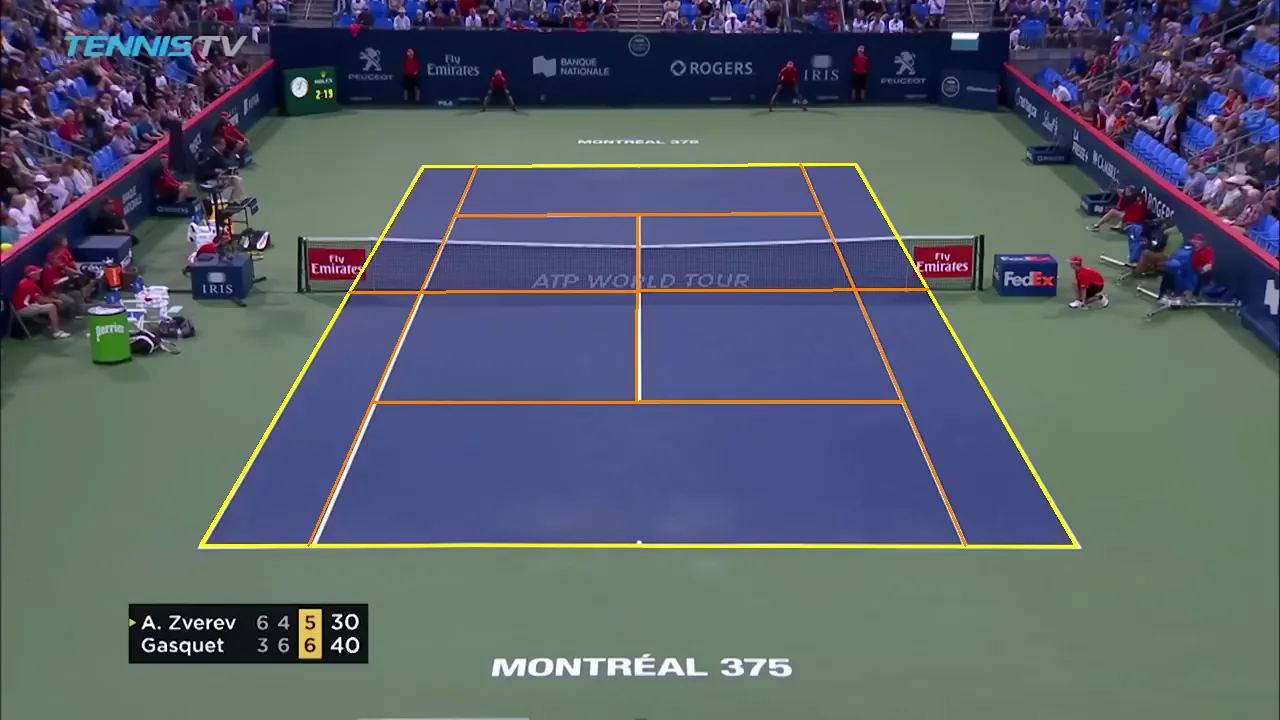
Yellow: the four lines the fit used. Orange: lines the fit had never seen. Mean error on the held-out lines: 0.0 to 0.8 pixels.
Sub-pixel, from four corners, on the first try. I had a refinement step planned and deleted it.
One detail in that image I keep looking at: the model's "net line" is the net's ground projection — dead straight — while the real net tape sags visibly above it. The court is geometry; the net is physics.
Pixels to meters
Now the payoff. Take M0's ball track, push every point through the homography, and draw it on a to-scale court:
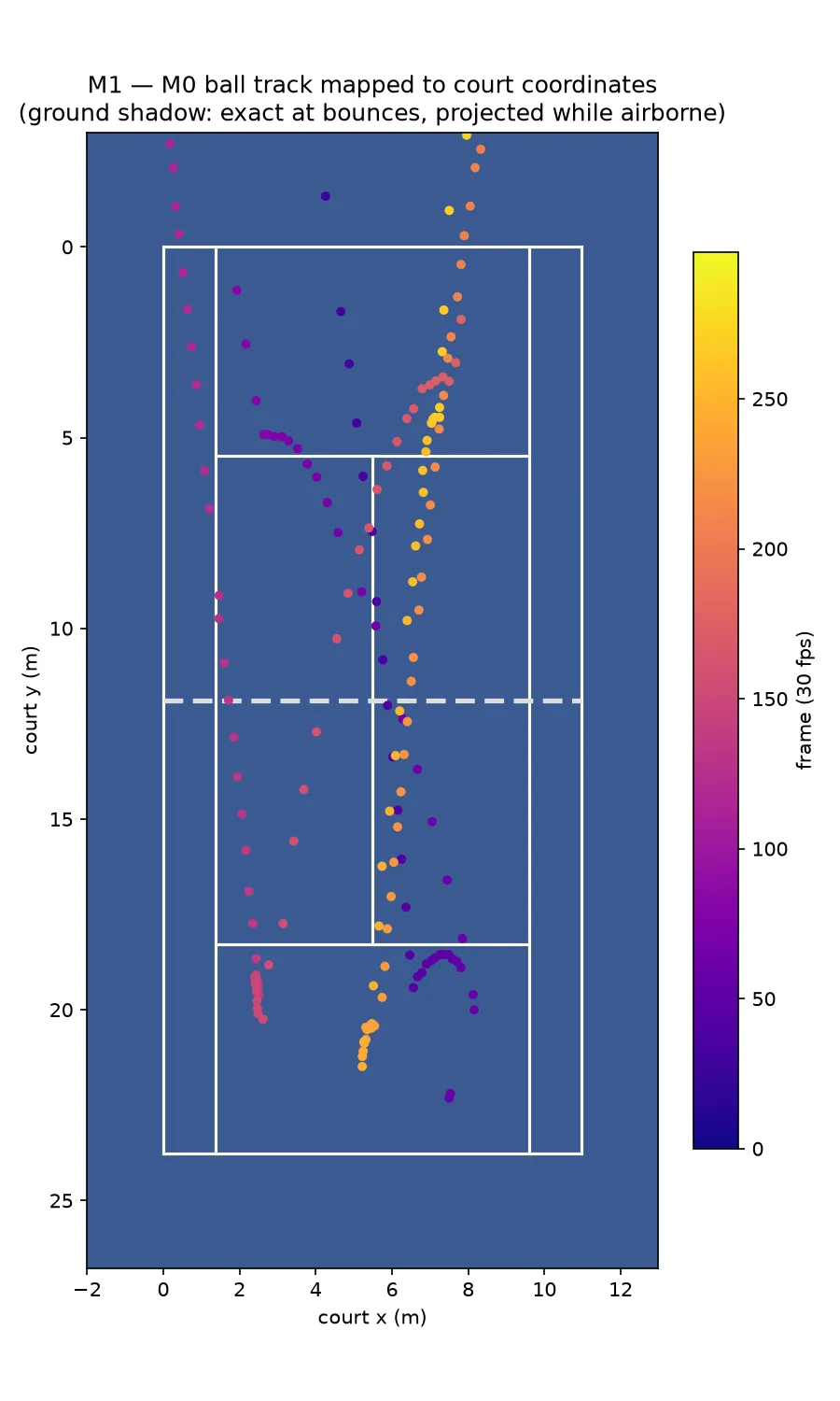
The M0 rally, seen from above for the first time. Color is time.
You can read the rally in it — crossings at the net, clusters near the baselines where the ball is struck low. And you can also read the catch: some points project 18 meters past the far baseline. That's not a fit error — the held-out lines just proved the homography is sub-pixel. It's physics again: a homography maps the ground plane, and the ball is airborne most of the rally. What this chart shows is the ball's ground shadow. The shadow is exactly right at the moments the ball touches the ground, and increasingly wrong the higher it flies.
Which is the cleanest possible handoff to M2: find the bounces. At a bounce, shadow equals truth — and the M0 trajectory already showed the bounces as sharp reversals begging to be detected.
The verdict
M1: done. Every step — clean plate, line detection, corner fit, validation — ran with no manual input and no API calls. Total cost: $0.00.
I can't stop thinking about the asymmetry. Tracking a fuzzy 8-pixel ball — the problem that used to be a research career — took a hosted billion-parameter model and a human click to bootstrap it. Finding the court and converting to real-world coordinates — the part that sounds like "computer vision" — took a median, a threshold, and four intersections. The hard and easy problems traded places when I wasn't looking.
Next, M2: hits and bounces. The trajectory is a series of smooth arcs interrupted by discontinuities, and every discontinuity is a hit or a bounce. Time to find out if that sentence survives contact with the data.